Mathematics of Computer Graphics Pt. 1

If you've seen my GitHub Page, you may have noticed I've had an interest in computer graphics for a while now. I have developed my programming abilities but writing and rewriting graphics engines, the one I'm most proud of being SGAL. All of these render engines have been done using OpenGL, which is a beast all of its own.

My most recent interest in computer graphics, however, has been raytracing and voxels (see my newest project). In order to get software like this to run efficiently the graphics card must be used as much as possible. Thus, compute shaders are a must. However, Apple has stopped supporting OpenGL on their devices since version 4.1 and compute shaders were introduced in version 4.3. This bit of bad news means that developing a legitimate cross-platform rendering engine requires using a more universally accepted framework. Luckily there's Vulkan. Using this framework, however, is going to be a big feat.

All of this to say, I hope to work up to discussing raytracing, raymarching, and efficient voxel rendering algorithms at some point, but I figured why not discuss the basics. What does it mean to render things?

The Basics of Rendering

The objective of rendering is simple in nature, but a little more difficult in practice. The ultimate function of rendering is very similar to how perception occurs in the real world. If there is an object in the world, its position can be represented (assuming we're discussing a Euclidean geometry where time is absolute) using three coordinates. However, when we view an object, its position can really represented by two coordinates relative to our center of vision. If two objects are in front of each other, we could only tell them apart by comparing their relative size in our view (due to the parallax effect). If they were dimensionless (say a point instead of a spatially extended object) and they were at the center of our vision, they would be indistinguishable.

This little fact is important and what it states is this: Information is actually lost because we are projecting a three-dimensional world down into the two-dimensional plane of our vision.

Projection

That word is important enough to warrant its own section here. We can demonstrate what we mean when we say project by messing around with some vectors.

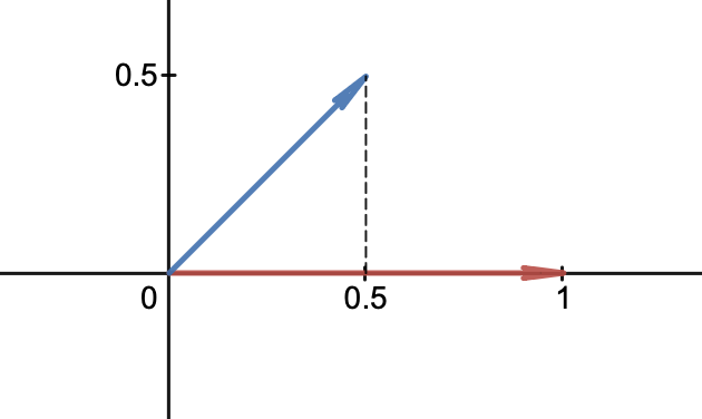
We can write the vectors shown above in component form as $\mathbf{r} = \hat{\mathbf{x}}$ and $\mathbf{b} = 1/2(\hat{\mathbf{x}} + \hat{\mathbf{y}})$ for the red and blue arrows respectively. We can imagine the red arrow as being the screen (it's just one dimensional in this case, that is all the points on the $x$-axis) and the plane being the space of our objects. If we think about the screen "seeing" the blue arrow, we would need to project it onto the screen. That is, project $\mathbf{b}$ onto $\mathbf{r}$.

We can do this by finding the component of $\mathbf{b}$ in the direction of $\mathbf{r}$. The dotted line makes $\mathbf{b}$ into a right triangle. Using some trig, we can find the component of $\mathbf{b}$ in the direction of $\mathbf{r}$ by multiplying the length of $\mathbf{b}$ by the cosine of the angle between $\mathbf{r}$ and $\mathbf{b}$. This gives us the length of the component of $\mathbf{b}$ in the direction of $\mathbf{r}$. That is $$ \text{Proj}_\mathbf{r}(\mathbf{b}) = |\mathbf{b}|\cos(\theta). $$ This would then give us the one-dimensional coordinate that the tip of $\mathbf{b}$ would be at on our one-dimensional screen. Let's try to compute this. We see that $|\mathbf{b}| = \sqrt{2}/2$, but what is $\cos(\theta)$? We could attempt to find $\theta$ using an inverse trig, but let's use another fact we know from vector calculus: $$ \mathbf{r}\cdot\mathbf{b} = |\mathbf{r}|\,|\mathbf{b}|\cos(\theta) \implies \frac{\mathbf{r}\cdot\mathbf{b}}{|\mathbf{r}|\,|\mathbf{b}|} = \cos(\theta). $$ This means our projected coordinate is $$ \text{Proj}_\mathbf{r}(\mathbf{b}) = \frac{\mathbf{r}\cdot\mathbf{b}}{|\mathbf{r}|} $$ We can compute these easily: $$ \begin{split} \mathbf{r}\cdot\mathbf{b} &= (\hat{\mathbf{x}})\cdot\left(\frac{1}{2}(\hat{\mathbf{x}}+\hat{\mathbf{y}})\right) \\ &= \frac{1}{2}(\hat{\mathbf{x}})\cdot\left(\hat{\mathbf{x}}+\hat{\mathbf{y}}\right) \\ &= \frac{1}{2}\hat{\mathbf{x}}\cdot\hat{\mathbf{x}}+ \frac{1}{2}\hat{\mathbf{x}}\cdot\hat{\mathbf{y}} \\ &= \frac{1}{2}. \end{split} $$ As we can see from the graph, $1/2$ is precisely where the dotted line connects to our screen. This kind of rendering method is called orthographic due to the fact that the dotted line is perpendicular to the screen. A consequence of this is visualized in the math above. If we were to increase the $y$ component of $\mathbf{b}$, it would not effect its position on the screen (since the orthogonal components $\hat{\mathbf{x}}$ and $\hat{\mathbf{y}}$ always have a vanishing dot product). This is against our intuition, since objects that move further away "get smaller." So what kind of projection do we need in order to take this phenomena into account?

One-Dimensional Perspective

The key difference is that our eyes act as a focal point, not a plane, in space. If we projected everything down to a point, we'd be left with no information, so that isn't very helpful. But, we can construct a focal point that is set back from the plane coupled with a field of view (FOV) measure.

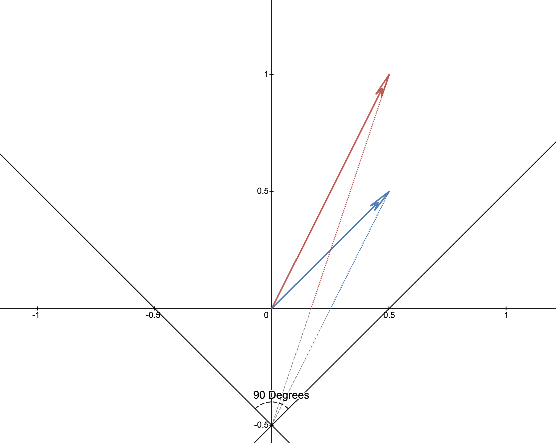
An example of this model is shown in the figure above, the point is set back by $1/2$ units and has an FOV of $\pi/2$ radians (or 90 degrees). The red vector is now simply the blue vector moved away in space and, as you can see by the intersection point with $y=0$ (the screen again), it is closer to the origin. This means that as the $y$ component of points goes to $\infty$, the projected coordinate goes to zero. This is the kind of behavior we would expect, as it is the behavior we observe in our every day lives.

How do we do this mathematically, though? How can we find these coordinates?

Let's move everything to the origin, then we can construct a line that goes through the origin and touches the point. The slope is simply the rise over the run: $$ y = \frac{r_y + n_{ear}}{r_x}x $$ where $n_{ear}$ is how far away the plane is, before it was how far set back from the origin the point is. We can solve for the $x$ value by setting $y = n_{ear}$ and solving: $$ n_{ear} = \frac{r_y + n_{ear}}{r_x}x \implies \frac{n_{ear}r_x}{r_y + n_{ear}} = x. $$ Notice, though, that the coordinates of edges of the screen might vary based off of $n_{near}$. We would like to normalize them to be between $-1$ and $1$. This is where the FOV comes in. Notice in the figure above that the intersections of the frustum with the $y=0$ line occurs as an opposite side to a right triangle where the adjacent side is simply $n_{near}$. Since the entire angle from left to right is $\theta$ (notice the dotted circle at the bottom), the angle for the right triangle is $\theta/2$. Thus, we can write $$ \tan\left(\frac{\theta}{2}\right) = \frac{x_{max}}{n_{near}} \implies x_{max} = n_{near}\tan\left(\frac{\theta}{2}\right). $$ Therefore, our screen coordinate $c$ is $$ c_x = \frac{x}{x_{max}} = \frac{r_x}{\tan\left(\frac{\theta}{2}\right)(r_y + n_{ear})}. $$ This is good, but we want to put it in a more convenient form (which will be discussed more later), so we can make an approximation where we say that $r_y + n_{ear} \approx r_y$ since $n_{ear}$ is more than likely a small number. Thus $$ \tag{1a} c_x = \frac{x}{x_{max}} = \frac{r_x}{r_y\tan\left(\frac{\theta}{2}\right)}. $$

We can also normalize $r_y$ to be between $0$ and $1$ which introduces the idea of a far plane. Values of $y$ that are greater than the far plane will assume values greater than one and, for most renderers, be excluded from rendering. We can do this with $$ \tag{1b} c_y = \frac{r_y - n_{ear}}{n_{far}-n_{near}} $$ This does what we want because when $r_y = n_{near}$, $c_y = 0$ and when $r_y = n_{far}$, $c_y = 1$.

Bring in the Linear Algebra

Now, how can we combine eqs. (1a) and (1b) into one form? We can utilize matrices and linear algebra. We wish to turn the vector $\mathbf{r}$ into the vector $\mathbf{c}$. We can do this using a matrix. If we have $$ \begin{pmatrix} 1/\tan(\theta/2) & 0 \\ 0 & 0 \end{pmatrix} \begin{pmatrix} r_x \\ r_y \end{pmatrix} = \begin{pmatrix} r_x/\tan(\theta/2) \\ 0 \end{pmatrix} $$ This is the $x$ component of $c$, but without the $r_y$ in the denominator. There's no way to divide out in matrix multiplication, so we need to store this value so that we can divide it out after this. This means we need to add a dimension to our matrix $$ \begin{pmatrix} 1/\tan(\theta/2) & 0 & 0 \\ 0 & 0 & 0 \\ 0 & 1 & 0 \end{pmatrix} \begin{pmatrix} r_x \\ r_y \\ 1 \end{pmatrix} = \begin{pmatrix} r_x/\tan(\theta/2) \\ 0 \\ r_y \end{pmatrix} $$ Putting a $1$ in our $\mathbf{r}$ vector is now convenient, since we need to add a constant to get (1b). That is, if we add to our matrix the first part, we get $$ \begin{pmatrix} 1/\tan(\theta/2) & 0 & 0 \\ 0 & (n_{far}-n_{near})^{-1} & 0 \\ 0 & 1 & 0 \end{pmatrix} \begin{pmatrix} r_x \\ r_y \\ 1 \end{pmatrix} = \begin{pmatrix} r_x/\tan(\theta/2) \\ \frac{r_y}{n_{far}-n_{near}} \\ r_y \end{pmatrix} $$ so that, to complete (1b), we utilize the constant: $$ \begin{pmatrix} 1/\tan(\theta/2) & 0 & 0 \\ 0 & (n_{far}-n_{near})^{-1} & -n_{ear}(n_{far}-n_{near})^{-1} \\ 0 & 1 & 0 \end{pmatrix} \begin{pmatrix} r_x \\ r_y \\ 1 \end{pmatrix} = \begin{pmatrix} r_x/\tan(\theta/2) \\ \frac{r_y - n_{ear}}{n_{far}-n_{near}} \\ r_y \end{pmatrix}. $$ Now, all we have to do is divide the $x$ component by $c_z$. We thus have a matrix that does our transformation for us, this is the projection matrix. Now, all we need to do is this, but in three dimensions.